Grouping data by month in Excel is a common task, especially when dealing with large datasets that need to be organized for reporting or analysis. While Pivot Tables are a powerful tool for this, they can sometimes be overkill or confusing to users who just want a simple, straightforward solution. Fortunately, Excel offers alternative methods that allow you to group data by month without the complexity of Pivot Tables. In this guide, we’ll explore these methods, showing you how to efficiently manage your data while maximizing Excel’s capabilities.
Why Avoid Pivot Tables?
Pivot Tables are a great feature in Excel, but they can be daunting for those who are not familiar with them. They require understanding how to drag and drop fields, configure settings, and sometimes involve troubleshooting when the data doesn’t appear as expected. For simpler tasks like grouping data by month, using formulas and built-in Excel features can be faster and more intuitive.
Method 1: Using Excel’s TEXT Function
The TEXT function is an underutilized feature in Excel that allows you to format dates in any way you prefer. Here’s how you can use it to group data by month:
- Add a New Column: Start by adding a new column next to your date data.
- Use the TEXT Function: In the new column, enter the following formula:
=TEXT(A2, "mmmm")
This formula converts the date in cell A2 to the full month name (e.g., “January,” “February”). - Copy the Formula Down: Drag the formula down to apply it to all rows. Now, you have a column with the month names extracted from your dates.
- Group Data: You can now sort or filter your data by this new column, effectively grouping your data by month without a Pivot Table.
This method is particularly useful if you need a quick, readable format for your data. It’s simple and doesn’t require any advanced Excel knowledge, making it accessible for all users.
Method 2: Using the MONTH Function
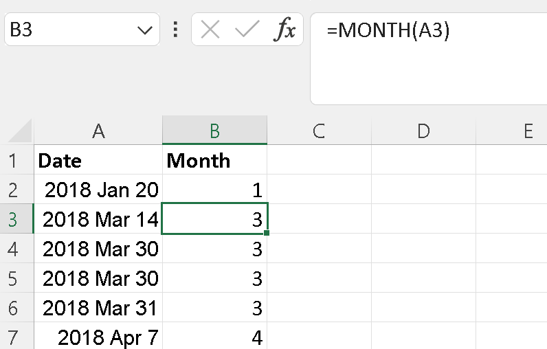
Another effective method is the MONTH function, which extracts the month number from a date. This method is great for scenarios where you need to perform calculations based on the month.
- Add a New Column: As with the TEXT function, add a new column next to your date data.
- Use the MONTH Function: Enter the following formula in the new column:
=MONTH(A2)
This formula will return a number from 1 to 12, corresponding to the month of the date in cell A2. - Copy the Formula Down: Apply the formula to all relevant rows.
- Group Data by Month Number: You can now sort or filter your data by this column, grouping it by month number.
This method is particularly useful if you need to perform further calculations, such as summing or averaging values by month. Since the result is a number, it’s easy to incorporate into other formulas or charts.
Method 3: Using an Array Formula
For those who are more comfortable with Excel, an array formula offers a dynamic way to group data by month. This method is particularly useful when working with large datasets or when you want to create a summary table.
- Create a Unique List of Months: First, create a list of unique months from your data. You can use the
UNIQUEfunction (available in Excel 365 and Excel 2019) or manually list the months. - Use the SUMIFS Function: In a new column, use the
SUMIFSfunction to sum values based on the month:=SUMIFS(B:B, A:A, ">=" & DATE(2021,1,1), A:A, "<" & DATE(2021,2,1))
This example sums values in column B where dates in column A fall in January 2021. - Apply the Formula for Each Month: Repeat the formula for each month, adjusting the dates as necessary.
Array formulas can be a bit tricky to master, but they offer powerful capabilities for those who need to perform more complex data analysis.
Method 4: Using Conditional Formatting
While not strictly a method for grouping data, conditional formatting can visually group your data by month, making it easier to analyze.
- Select Your Data Range: Highlight the date column you want to format.
- Apply Conditional Formatting: Go to the Home tab and select Conditional Formatting > New Rule. Choose “Use a formula to determine which cells to format.”
- Enter the Formula: Use a formula like
=MONTH(A2)=1to apply a format to all dates in January, for example. - Repeat for Each Month: Set up similar rules for each month, using different colors to distinguish them.
This method is useful for quickly identifying patterns or trends in your data, though it doesn’t physically group the data like the other methods.
Conclusion
Grouping data by month in Excel without a Pivot Table is not only possible but also often preferable for users looking for a more straightforward approach. Whether you use the TEXT function for a quick fix, the MONTH function for numerical analysis, array formulas for advanced tasks, or conditional formatting for visual grouping, Excel offers multiple ways to achieve your goal. By mastering these techniques, you can streamline your workflow and make data analysis more efficient and accessible.
Try these methods the next time you need to group data by month, and see how much simpler Excel can become without relying on Pivot Tables.
To get things done even faster, see my other post on the best Excel keyboard shortcuts.